What is Monte Carlo retirement simulation?
Monte Carlo runs many random market paths and checks how often your spending rule lasts. In SuperCalc Pro’s Advanced Calculator each path year draws a random historical year (returns and CPI together) from the 1928-2025 series, then that sits beside full historical replay on the same balance, fees, drawdowns, and Age Pension settings.
What the calculator does: typically 1,000 Monte Carlo trials that resample historical years with replacement, plus a rolling historical backtest across every start year that fits your horizon. Same Australian rules in both modes.
Why both matter: historical replay answers “would this spend have survived 1973 or 2008 in the order markets actually delivered?” Monte Carlo answers “how often do remixed historical magnitudes still fund the same spend?” Tools that only show a constant 7% path do neither. Tools that only show a normal-distribution Monte Carlo never reuse the real crash sizes in your dataset.
Important: General information only, not financial product advice. SuperCalc Pro does not hold an Australian Financial Services Licence (AFSL). The article does not recommend opening, closing, or changing any super fund or product. Seek advice from a licensed financial adviser, SMSF specialist, or accountant as appropriate.
Financial software loves the phrase “Monte Carlo simulation.” It sounds rigorous. Often what sits behind the label is a parametric draw: normally distributed returns, independence year to year, a chosen mean and volatility. That is a different machine from resampling real historical years. For Australian retirees the useful question is not “Monte Carlo yes or no” but which generator produced the paths, and whether you also look at ordered historical replay where crashes arrive in the clumps markets actually delivered. For how marketing labels compare to mechanics, see Monte Carlo versus reality.
This article explains both industry-standard parametric Monte Carlo and what SuperCalc Pro actually runs, contrasts that with historical backtesting, and embeds empirical success rates from the same sustainability engine as the safe withdrawal rate Australia tables (balanced preset, fees in code, single homeowner pension from 67). Those historical percentages are not Monte Carlo draws. They are the frequency of success across real ordered return paths.
Rule of thumb: If someone shows a “probability of success” without listing how returns are simulated, whether spending is indexed, and whether Age Pension is modelled, you do not yet know what the percentage means.
What Monte Carlo retirement simulation actually does
In retirement software, “Monte Carlo” can mean at least two different generators:
- Parametric: each year draws a return from a fitted distribution (often normal) with a mean and volatility you choose. Crash magnitudes are whatever that bell curve allows.
- Historical bootstrap (what SuperCalc Pro’s Advanced Calculator does): each year of each trial picks one random calendar year from the stored series (1928-2025), with replacement. That year’s multi-asset returns and Australian CPI travel together into the portfolio return. Default is 1,000 trials.
Those are not interchangeable. A normal curve centred on ~8% with ~12% vol will understate how often history actually delivered 1929-, 1973-, or 2008-sized years. Bootstrap keeps those magnitudes in the draw pool. What it does not keep is the original order: SuperCalc Pro draws single years independently (not multi-year blocks), so momentum and volatility clustering can still be broken apart. That is a milder version of the same independence problem as parametric Monte Carlo: better on crash size, not a full fix on sequencing. Ordered historical windows on the same inputs are the check against that blind spot.
Conceptually, one SuperCalc Pro trial looks like this:
- Start with $500,000 at age 67
- For year 1, draw a random historical year from the dataset (say 1974) and apply that year’s allocation-weighted returns and inflation
- Subtract annual spending (e.g. $55,000 in today’s dollars, with the engine’s indexing rules)
- Check Age Pension eligibility, add any entitlement
- Repeat for all 28 years, drawing a new historical year each step (draws can repeat)
- Record: did money last to the horizon?
- Repeat the whole chain 1,000 times
- Count successes: e.g. “730 paths didn’t run out = 73% success” under this resampling process
Strengths: you see a spread of outcomes, not a straight-line 7%. Tail years in the cloud are built from returns that actually occurred in the dataset. You can stress spend, horizon, and allocation quickly.
Weaknesses (of any independent-year bootstrap): scrambling years breaks real clustering. Markets show momentum, volatility clustering, and regime shifts, the article’s earlier point about “nice” vs “chaotic” sequences still applies when years are drawn independently, even if each year’s return is a real historical observation. Ordered historical replay is the check against that blind spot.
Historical simulation as a complementary “probability”
Historical simulation asks a different question: If I had retired in 1928, 1929, … through to the last year that fits a full horizon, would my fixed strategy have survived? Count successes, divide by paths. That ratio is sometimes called a success rate. It is not the chance your retirement will fail next decade. It is how often the past contained a friendly ordering for your spending rule.
The underlying series in code runs 1928-2025 (98 calendar years). For a 28-year horizon that is 71 valid start years (1928 through 1998). The success-rate table below uses that full panel from the same sustainability engine as safe withdrawal rate Australia: age 67, $500,000 super, pension on, balanced preset. Success means maximum sustainable real income on that start year clears the stated spend (within a small dollar tolerance).
Not comparable to earlier published versions of this table. Figures here were regenerated on 10 August 2026 against the current Fixed MSI engine on all 71 starts (1928–1998), shared with safe withdrawal rate Australia and super drawdown strategy Australia. Earlier July 2026 versions used the same window with older rate stacks; still-older pages used a 70-start panel. Treat this as a corrected shared panel, not a one-year sample-size tweak.
| Fixed annual spend | Paths succeeded | Historical success rate |
|---|---|---|
| $45,000 | 71 / 71 | 100% |
| $50,000 | 64 / 71 | 90% |
| $55,000 | 53 / 71 | 75% |
| $60,000 | 33 / 71 | 46% |
Think of this table as ordered history, not Monte Carlo: the paths are the actual sequences investors lived through. Monte Carlo in the Advanced Calculator asks how often remixed historical years still fund the same spend.
Sequence risk, Monte Carlo, and Australian super
Sequence of returns risk is the interaction of withdrawals with bad timing. Ordered historical replay preserves that timing. Bootstrap Monte Carlo keeps historical return magnitudes but remixes order year by year. Parametric Monte Carlo may miss both the real crash sizes and the clustering. The cost of pure history is a finite sample: you only get as many full windows as the dataset allows.
For Australians, add means-tested Age Pension, minimum drawdown rules, and franking-aware equity returns where configured. A US-centric Monte Carlo may ignore entitlements entirely. SuperCalc Pro applies pension and fees inside the same sustainability loop for historical and Monte Carlo modes.
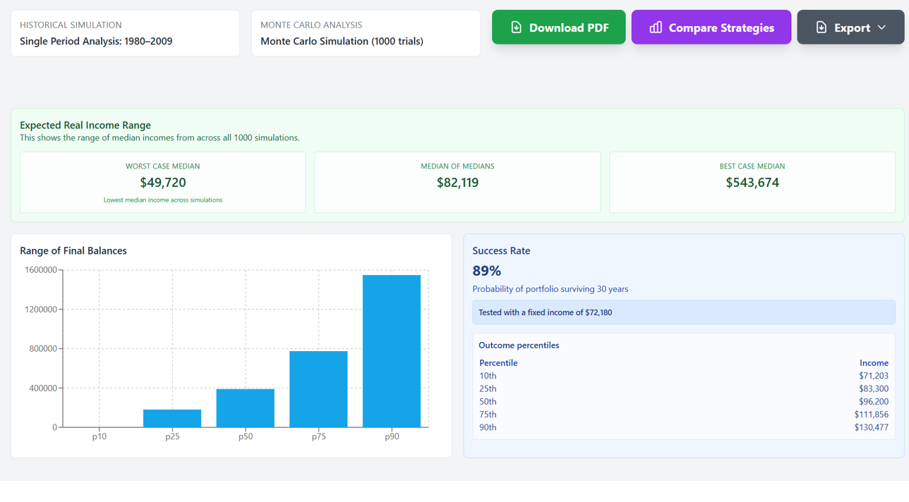
Maximum sustainable income: what Monte Carlo hides in the tails
Most Monte Carlo tools show one number: "X% of paths succeed at $55,000 spend." But that hides crucial detail. A more honest analysis: for each simulated path, how much could you actually spend and still reach end-of-life? This flips the question from binary success/fail to a distribution of feasible spending.
Running this style of analysis on 1,000 bootstrap paths (balanced fund, $500,000 starting balance, age 67, 28-year horizon, with Age Pension), the useful output is a spread of maximum sustainable spending, not a single success percentage. In one illustrative run the shape looked roughly like this (your screen will differ with fees, allocation, and random seed):
- Lower tail (around the 10th percentile): spending in the high-$40k to low-$50k range
- Middle of the pack: spending somewhere in the mid-to-high $50k range
- Upper tail (around the 90th percentile): spending into the mid-$60k range or higher
That spread is the point. A tool that only says “about three-quarters of paths succeed at $55k” can be true and still incomplete. It does not tell you how tight the margin is on the bad draws, or how much headroom lucky paths would have had.
Upside tails feel comforting and rarely change how much you actually spend. Downside tails force a choice: spend less, lean harder on Age Pension, or accept a higher chance of running down too early. A useful Monte Carlo view surfaces that asymmetry instead of hiding it behind one percentage.
Comparison: What does a higher fixed-income allocation look like?
Shift toward more bonds, say 40% Australian shares, 20% international, 40% fixed income instead of a heavier equity mix, and expected return and volatility both drop. In practice the middle of the spending distribution usually moves down more than the worst tail improves. You often buy steadier ordinary years, not insurance against the truly ugly sequences where equities and bonds get hit together.
That is the trade-off worth seeing on your own inputs: less median spending capacity for smoother mid-path behaviour, without assuming the left tail magically disappears. Open the Advanced Calculator and change the allocation once; the cloud will tell you whether the defensive mix is buying what you hoped.
When Monte Carlo is still worth running
Despite caveats, Monte Carlo remains useful for sensitivity analysis. Change spending, retirement age, allocation, or pension assumptions and watch the cloud of remixed-history outcomes move. Good tools make those perturbations easy. The mistake is treating one default success rate as the probability.
A worked sensitivity example
Suppose you run 1,000 historical-bootstrap trials on a balanced allocation with $55,000 annual spending and see about 73% success. Now change one knob. The directional shifts below are illustrative of the pattern: not a guarantee of what your screen will show, but they match the kind of sensitivity the Advanced Calculator is built to surface.
- Spend $5,000 more: often the biggest swing. Spending is the lever you actually control.
- Retire two years earlier: longer drawdown, thinner margin, horizon risk compounds.
- More defensive allocation: median capacity usually falls; the left tail may not improve as much as you hope.
- Weaker Age Pension assumption: Australian plans that lean on the pension in the tail can look fine until that support is cut in the model.
- Compare to ordered history on the same spend: if Monte Carlo success is high but historical success is low (or the reverse), dig into which sequences are driving the gap before you raise spending.
To see real numbers: open the Advanced Calculator and change one assumption at a time on your own inputs. That beats any generic list of percentage-point moves.
You are not forecasting. You are asking what breaks the plan. If success stays above a floor you can live with across those shifts, the plan has some resilience. If one small change collapses it, spending or risk needs another look.
What usually moves the needle
In practice, for Australian drawdown plans in this kind of model, the ranking is often:
- Spending level: the clearest lever you control.
- How long you draw: retiring earlier or living longer.
- Allocation: shifts the cloud; does not erase sequence risk.
- Age Pension assumptions: easy to underweight until you turn them down in the model.
- Whether you check ordered history: bootstrap Monte Carlo alone will not show you 1973-in-calendar-order.
That is why Monte Carlo is most useful when you reframe the question from “will I succeed?” to “what spending level still looks acceptable when I stress the assumptions I care about?”
For a longer discussion of disagreements between methods, see Monte Carlo versus reality and probability retirement fails Australia (failure-rate framing of the same historical counts).
Red flag: If Monte Carlo success is high but historical success for the same spend is low, your Monte Carlo engine may be too optimistic (or your historical test too harsh). Investigate before relaxing spending.
The tension between scepticism and the tool itself
I should be direct about the conflict: this article spends most of its space arguing for caution with Monte Carlo, listing its limitations, and championing historical backtesting. Then it points you toward a calculator that includes a Monte Carlo mode. That’s worth acknowledging.
The honest answer is that Monte Carlo is neither useless nor magic. It's most valuable when used as sensitivity analysis. Not as a forecast, but as a machine to ask "what breaks my plan?" If your retirement plan survives when you perturb every major assumption, it's robust. That requires comparing Monte Carlo and historical results on the same calculator, seeing where they diverge, and asking why. The tool works when it reveals model risk, not when it hides it.
A calculator with both Monte Carlo and historical backtesting modes allows that comparison. Tools with only one method, whether Monte Carlo or historical, are incomplete by design.
Australian-specific Monte Carlo gotchas
Many Monte Carlo tools in the retirement space were built for US planning (Social Security, Roth conversions, 4% rule) and retrofitted for Australia. That creates blind spots.
1. Age Pension means-testing isn't a straight line
Your Age Pension drops as assessable assets and income rise, and the taper is rule-based rather than a vague “less pension when richer.” Paths that deplete super faster can become eligible for more pension later, a feedback loop many simplified Monte Carlo tools skip. SuperCalc Pro applies Centrelink-style means tests inside the sustainability loop; always confirm current thresholds before acting.
2. Franking credits matter for returns, not just tax chats
Some Monte Carlo models fit a return distribution that never really accounts for franking. SuperCalc Pro’s bootstrap paths use the Australian share sleeve from the historical series, with franking credit boost applied where you set the franking percentage. Treat a generic “8% forever” assumption as a blunt instrument until you know what sits behind it.
3. Superannuation withdrawal rules shift with age
Legislative minimum drawdowns rise with age bands. A long retirement spans more than one regime. A Monte Carlo that lets you pick any withdrawal every year without a minimum floor may be too flexible relative to how account-based pensions actually work.
4. Longevity for couples is not a single-life table
Australian life expectancy is high. A 28-year horizon from 67 is conservative for a median single retiree and still not extreme for a couple where one partner may live longer. If the tool only models one life, you can understate how long the household needs money. Prefer a horizon you would still be comfortable explaining to a sceptical spouse, then stress spending against that finish line.
5. Currency and international equity returns
Unhedged international equities bring a currency layer. Some retail Monte Carlo setups ignore it. SuperCalc Pro’s paths use the stored international sleeve for each historical year drawn; when you compare tools, ask whether currency is inside the series or assumed away.
Run Monte Carlo and historical simulation together
Start on the free Monte Carlo calculator landing for how the two lenses differ. Same balance, fees, and Age Pension settings open in the app next.
Monte Carlo Calculator LandingBottom line
Monte Carlo in SuperCalc Pro is a historical-year bootstrap stress machine: change spending, allocation, retirement age, or pension assumptions and watch the remixed cloud move. The headline success rate alone is not a prophecy, it is probability under that resampling process.
Pair it with ordered historical backtesting on the same inputs. When they disagree, that gap is information. When a tool only offers a constant return forever, or a normal curve that never saw 1973, you never get either view honestly labelled.
What it costs to keep modelling
Start on the free Monte Carlo calculator landing. Run Advanced Retirement free next. Unlimited scenarios, historical stress tests, and PDF exports are $149 a year, or $14.99 a month if you’d rather not commit upfront, typically less than one hour of paid advice for the same modelling work.
Run the Advanced Calculator →No card required to try it. Subscribe only if the model is useful enough to keep using.
Disclaimer: General information only, not financial product advice or personal advice. SuperCalc Pro Pty Ltd does not hold an Australian Financial Services Licence (AFSL). This article does not recommend opening, closing, or changing any super fund or product. Simulation results depend on inputs and methodology. Past data does not predict future performance. Government rules and rates change. Verify current rules with official sources and seek advice from a licensed financial adviser before altering your retirement strategy.