Important: This article is general information only. It is not personal financial advice, not financial product advice, and not a recommendation to buy, sell, or switch investments. SuperCalc Pro does not hold an Australian Financial Services Licence. The figures below are indicative modelling outputs, not promises about what markets will do next.
Every market cycle produces the same argument in a fresh costume. One side says the market always finds a reason to stay expensive. The other says long-run valuation still matters and the price eventually comes back toward trend. The attraction of a regression-to-the-mean estimate is obvious: it turns that argument into a number. Fit a log trend through the market's history, look at where the index sits today, then ask what annual return would bring it back to the line in ten years.
Cleaner than a hot take and less mystical than a strategic outlook deck, but it raises an awkward question. If the method is good, it should have done a respectable job on past windows. If it fails badly when tested on history, the neatness of the number is not the same thing as reliability. The rolling regression tool exists to answer that question, and it is the right way to treat any return estimate, whether it comes from a simple chart fit or from a large institutional model.
What this method is actually doing
The method here is deliberately simple. It builds a synthetic index from annual total returns, converts that index to logs, then fits an ordinary least squares line over a chosen history window. If you choose a 50-year fit and a 10-year trial, the model asks a very specific question: given where the market sat at the end of that 50-year window, what real CAGR over the next 10 years would have been required to get the index back onto the fitted trend line by the test end?
Not the same thing as saying the market will deliver that return. It is a convergence number. It tells you what mean reversion would require if it happened on the timetable you chose. The distinction matters because a great many valuation arguments quietly smuggle in the assumption that expensive markets must fix themselves within a decade. History does not owe you that.
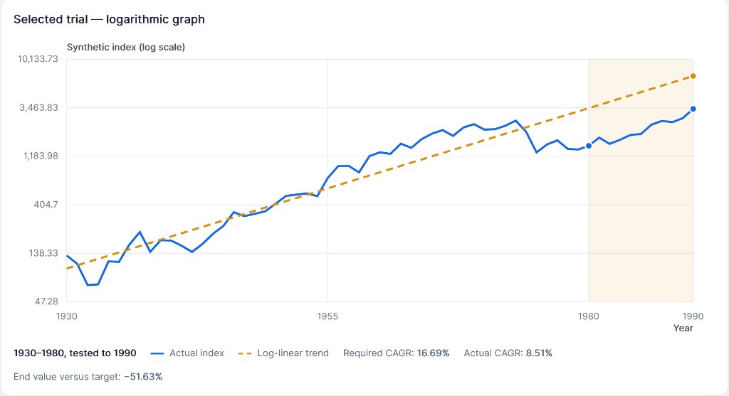
The regression chart makes the method visual: the blue line is the synthetic index, the dashed line is the fitted trend, and the shaded band is the test window where the required catch-up return is measured.
The historical backtest is the part that stops this becoming astrology
The first virtue of this approach is that it is falsifiable. You can roll the window forward and ask whether past forecasts would have worked. Across the full 50-year real S&P setup in the regression tool (39 completed 10-year trials from 1978 through 2016, stepping one year at a time) the mean absolute CAGR error is 3.66 percentage points a year. Actual returns came in above the required catch-up number in 21 of 39 windows and below it in 18, so the method does not systematically lean bullish or bearish. It just leans confident, which is not the same thing.
On direction, the hit rate is better. In 29 of 39 trials, the market moved the way valuation would suggest: when the index finished the fit window above its trend line, the subsequent 10-year real return came in below the fitted trend CAGR; when it finished below trend, returns came in above it. Seventy-four per cent — not proof, but a base rate worth reporting before cherry-picking individual windows. The three late-1990s endpoints (1998, 1999, 2000) sit at the extreme end of that distribution, with the market 78% to 121% above trend. All three flagged negative required CAGRs; two of three delivered negative actual 10-year returns, and the third barely scraped positive.
The other 10 windows got direction wrong, and the pattern is informative rather than random. Four endpoints — three in the late 1970s/early 1980s plus 2003 — had the market at or below trend, but subsequent returns still fell short of the fitted trend CAGR: catch-up that was real but too slow, or that never arrived. Four mid-1990s windows had the market at or slightly above trend while the subsequent decade kept compounding above trend anyway — momentum, not mean reversion. The remaining two (2014, 2015) were near-trend setups where the market simply kept running. Directional misses cluster in catch-up bull phases and momentum bull phases, not in the extreme overvaluation cases where the signal matters most.
At the other extreme, a 50-year real fit ending in 1978 implied that getting back to trend by 1988 would have required a real CAGR of 17.47% a year. The market actually delivered 6.11% real. The next two adjacent windows are not much kinder: 1929-1979 to 1989 required 17.51% real and got 7.17%; 1930-1980 to 1990 required 16.69% real and got 8.51%. Those are the kind of misses that matter if someone is pretending this method can pin down the next decade with precision.
None of this makes the method useless. The honest reading is narrower. A regression-to-trend estimate is better understood as a valuation anchor than as a forecast in the everyday sense. It tells you what the market would need to do to revert to a long-run line. It does not tell you that the market will choose to cooperate on your timetable.
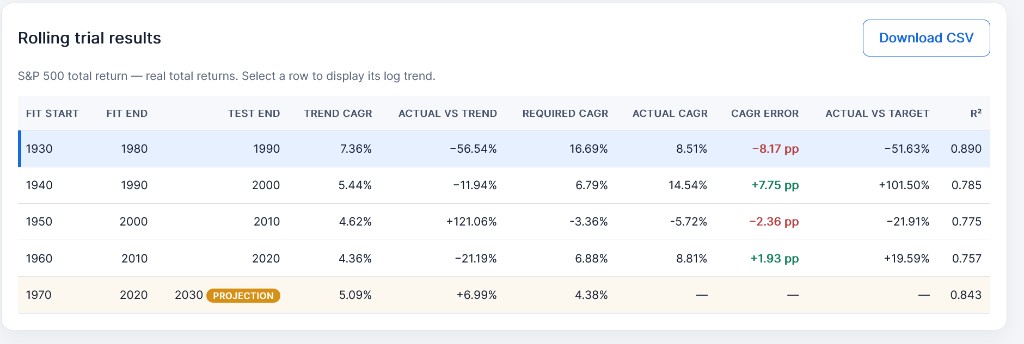
The rolling table is the useful part. It forces the tidy theory to answer a messy historical question: what happened next?
The present estimates are more moderate than the dramatic old backtests
Once you move the window forward to the present, the numbers settle down. In the current S&P 500 setup using real returns, a 50-year fit ending in 2025 implies a required real CAGR of 5.31% a year to get back to trend by 2035. Push the fit one year further so it ends at the 2026 synthetic index level, and the required real CAGR drops to 4.61% to get back to trend by 2036.
Here is the first useful practical observation. The estimate is not a dramatic doom number. It is a middling real return assumption, which is precisely why this framework can be helpful for planning. When the market is well above its own fitted line, the implied future real return usually softens. It gives you a cooler base case than the simple habit of extrapolating the last bull market forever.
Australian shares: the same method, run with the same discipline
For Australian readers, the U.S. backtest is instructive but not sufficient. The same 50-year real setup applied to Australian shares total returns produces 39 completed 10-year trials (1978–2016, stepping one year at a time). The mean absolute CAGR error is 1.89 percentage points a year — materially lower than the S&P's 3.66pp. Directional accuracy is weaker: 24 of 39 trials (61.5%) moved the way valuation would suggest, versus 74% for the S&P. Actual returns came in above the required catch-up number in 15 of 39 windows and below it in 24 — the required CAGR exceeded what actually happened more often than not, a modest optimistic tilt in the forecast.
The current projection is where the contrast with the U.S. is sharpest. A 50-year real fit ending in 2026 has Australian shares sitting 16.8% below their own fitted trend — the opposite sign from the S&P, which is currently above trend. The required real CAGR to get back to trend by 2036 is 9.09% a year on a 10-year trial. That is not a rounding error. It is a structurally different reading from the S&P's 4.61%.
Historical windows temper the "cheap Australian shares" narrative. The fit ending in 2016 — market 11% below trend — required 8.01% real to get back to trend by 2026. Actual was 6.27% real: a miss of 1.73pp a year, directionally right (below-trend market, needed catch-up, got moderate returns) but not close enough to call a win. The fit ending in 2007 had the market 40.5% above trend before the GFC; required 3.28% real, actual was 2.06% — directionally correct but again not precise. The fit ending in 1981 is the ugly one: market slightly below trend, required 8.38% real, actual was 2.81% — a 5.56pp-a-year miss in a period dominated by the early-1980s inflation shock and the 1987 boom-bust.
Two caveats belong next to any Australian number. First, the series is a synthetic total-return index built from annual returns in the SuperCalc Pro data file, not a direct All Ordinaries Accumulation Index feed — older years rely on the same dividend-yield approximations as the main calculator. Second, the Australian 50-year fit has a higher R² than the S&P (0.97 versus 0.91 at the current window), which can make the trend line look more authoritative than the underlying return data justifies. Treat the 9.09% as "what catch-up would require under these approximations," not as a forecast.
| Trial length | Required real CAGR | Forecast horizon |
|---|---|---|
| 5 years | 11.12% | 2026 → 2031 |
| 10 years | 9.09% | 2026 → 2036 |
| 15 years | 8.42% | 2026 → 2041 |
Shorter trials demand a sharper catch-up. The 5-year trial implies 11.12% real — two percentage points above the 10-year figure. For retirement planning, that sensitivity matters as much as the headline number.
The dot-com window: regression got the direction right
Within that 74% directional hit rate, the dot-com peak is the clearest win. The 50-year real S&P fit ending in 2000 had the market sitting 121% above its own fitted trend. The method was screaming that the index was absurdly extended. The required 10-year real CAGR to get back to trend was negative 3.36% a year. Negative. The model was not just cautious — it was saying the market needed to fall in real terms for a decade to get back to the line.
The actual 10-year real return from 2000 to 2010 was negative 5.72% a year. Two crashes, dot-com then the GFC, sandwiching a partial recovery that never got close to the 2000 peak in real terms. The regression method missed the magnitude (it expected a milder negative; reality was harsher), but it got the direction unambiguously right. At a time when plenty of professional forecasters were still publishing positive 10-year outlooks, the trend line was saying the market was so far above its own history that even getting back to normal meant going down.
The adjacent windows tell the same story. The fit ending in 1999 had the market 106% above trend and required negative 2.74% real; actual was negative 6.02%. The fit ending in 1998 had it 78% above trend, required negative 1.37% real, and the actual return scraped to positive 1.32%. Across the whole late-1990s cluster the directional signal was consistent: overvalued, expect real returns at or below zero for the next decade. Two of three delivered negative; the third barely cleared zero.
This does not prove the method always works. It does show the method can catch extreme overvaluations and flag them correctly as dangerous — the cases where a directional call matters most, even when the point estimate is wrong.
The 2016 window: Vanguard versus regression
The more recent comparison is instructive for a different reason. Both frameworks called for moderate returns. Both were wrong. But once you put them on the same real basis, the regression method was closer to what actually happened.
In Vanguard's 2017 Economic and Market Outlook (published December 2016, VCMM simulations as of September 2016), the text states global equities in a guarded 5%–8% nominal range (Figure II-4) and a 50% likelihood of a 5% average real return for a global equity portfolio over the decade to 2026 — against 6.8% real per year for 1926–2016. Figure II-6 shows nominal VCMM distributions for individual asset classes; the accompanying text states that U.S. equity was expected to fall short of both its own historical average and global ex-U.S. equity. The report does not state a single headline U.S. equity median in the body text — only that the U.S. distribution sits below global ex-U.S. in the chart.
The regression method at the same point — 50-year real S&P fit ending in 2016 — had the market about 5% below its own trend (actual vs trend: negative 4.96%). The required real CAGR to get back to trend by 2026 was 5.11% a year: roughly in line with Vanguard's 5% real global median, but notably higher than what a U.S.-specific reading of Vanguard's framework would imply. If U.S. equities were expected to underperform the global median by one to two percentage points in nominal terms, a 2%–2.5% inflation assumption puts the implied U.S. real forecast in the 2.5%–4% ballpark — material uncertainty, but directionally below the regression output.
What actually happened? The 10-year real CAGR from 2016 to 2026 was 9.38%. The market blew past the trend line by nearly 49%. On a real basis: the regression method's 5.11% required CAGR missed actual by 4.27 percentage points a year. Vanguard's 5% real global median missed by 4.38 points. A U.S.-specific reading of Vanguard's framework — perhaps 3%–3.5% real once you account for the stated U.S. underperformance versus global ex-U.S. — would have missed by roughly 6 to 6.5 points a year. The regression method was not right. It was, however, meaningfully closer to the outcome than a U.S.-tilted reading of Vanguard's own 2016 numbers.
The 2016–2026 decade was exceptional. AI-driven mega-cap re-rating, pandemic stimulus, and a sustained earnings boom produced a structural shift that none of the valuation-anchored models reviewed here predicted. Both frameworks were saying the same broad thing in 2016: expect moderate returns, not a barnstorming bull run. Both were wrong in direction. The regression method's error was smaller once you convert Vanguard to the same real terms.
The honest comparison (all real, 2016 → 2026): Regression required CAGR: 5.11% real (miss: 4.27 pp/yr). Vanguard global equity median: ~5% real per the September 2016 VCMM (miss: 4.38 pp/yr). Vanguard U.S.-tilted reading: ~3%–3.5% real, implied from stated U.S. underperformance (miss: ~6 pp/yr). Actual: 9.38% real. Neither model predicted the boom. The regression method was closer.
Where Vanguard's current outlook lines up
Vanguard's December 2025 Economic and Market Outlook — released 10 December 2025, VCMM simulations as of 31 October 2025 — puts expected U.S. equity returns at 4%–5% nominal annualised over the next 5 to 10 years, driven primarily by its assessment of large-cap technology valuations. The press release and published report both use that band. It is a nominal number. A later VCMM running (January 2026) widened the 10-year U.S. equity range to 3.9%–5.9% nominal — VCMM updates monthly, so treat the exact band as a snapshot, not a fixed forecast.
Strip roughly 2%–2.5% for expected inflation and Vanguard's December 2025 headline implies about 1.5%–3% real for U.S. equities. The current regression output for the S&P is higher: 4.61%–5.31% real (50-year fit ending 2025–2026, 10-year trial). Vanguard's model is more bearish on U.S. equities than the regression trend line — partly because it penalises the specific composition of current earnings and multiples, particularly AI-exposed mega-caps, rather than measuring distance from a long-run log trend.
AQR's 2026 Capital Market Assumptions (Exhibit 3, as of 31 December 2025) puts U.S. large-cap equities at 3.9% local real geometric return over 5–10 years — the lowest among major markets in that exhibit — using a yield-plus-growth model that explicitly assumes no mean reversion in valuations. Three different methods, three different frameworks — Vanguard nominal 4%–5% (Dec 2025), AQR real 3.9%, regression real 4.6%–5.3% — and the direction is similar even though the levels differ: none of them is saying the next decade looks like the last one.
Parameter sensitivity: the number moves more than you'd think
The single biggest weakness of a one-line OLS fit is not the maths. It is how much the output swings when you change the window. The tables below use the current S&P projection (real returns, fit ending 2026) and show required catch-up CAGR across fit length and trial length. The range is enormous.
| Fit period | 5-year trial | 10-year trial | 15-year trial |
|---|---|---|---|
| 30 years | −3.65% | −0.05% | 1.18% |
| 40 years | 0.89% | 3.01% | 3.72% |
| 50 years | 3.39% | 4.61% | 5.02% |
| 60 years | −0.97% | 1.91% | 2.88% |
Read that table carefully. The current S&P "headline" of 4.61% real (50-year fit, 10-year trial) sits in a band that runs from negative 3.65% to 5.02% depending on how you set the inputs. A 30-year fit with a 5-year trial says the market is so far above its shorter trend that catch-up requires negative returns. A 50-year fit with a 15-year trial says 5.02% real. Both are defensible outputs of the same method applied to the same data.
Historical rolling windows show the same fragility in the backtest itself. Shift the fit start year by one and the required CAGR moves even when the economic story has not changed:
| Fit window | Required real CAGR | Actual real CAGR | Forecast error |
|---|---|---|---|
| 1928–1978 → 1988 | 17.47% | 6.11% | −11.36 pp |
| 1929–1979 → 1989 | 17.51% | 7.17% | −10.34 pp |
| 1930–1980 → 1990 | 16.69% | 8.51% | −8.18 pp |
Three adjacent windows, three required CAGRs between 16.69% and 17.51%, three actual outcomes between 6.11% and 8.51%. The method is not producing a stable number. It is producing a number that is conditional on choices you made before you opened the spreadsheet.
The real risk is false precision
The biggest danger in this whole area is not pessimism. It is precision. Saying "the next decade will probably be softer than the last one because valuations are high" is a respectable broad statement. Saying "the correct real return for the next decade is 4.61%" is theatre unless you immediately add the caveat that the figure is conditional on a very specific path back to trend.
Markets can resolve valuation excess in many ways. They can grind sideways while earnings catch up. They can suffer a sharp multiple compression. They can stay expensive for longer than any sober person thinks possible. They can also be carried higher by a structural earnings shift that the fitted trend line does not yet know how to price. A backtest that misses by 8 to 11 percentage points a year on some historical windows should make anyone modest about point estimates.
The practical use: treat regression-to-the-mean as a planning anchor, not a prophecy. If your retirement plan only works when future real returns look like the last great bull market, that is a fragile plan. If it still works when you plug in a cooler valuation-aware number, you are on firmer ground.
How to use this without fooling yourself
The sensible use case is straightforward. Start with the regression estimate as one input, not the whole answer. If a current 50-year S&P fit says about 4.6% real on a 10-year trial, use that as a sober planning case — but run the sensitivity table first. If the same market reads anywhere from negative to 5% depending on fit length, your plan should survive the whole band, not just the middle cell.
For Australian shares, apply the same discipline. The 9.09% real headline on a 10-year trial is one cell in a table that runs from 8.42% to 11.12% depending on trial length, against a backtest with a 1.89pp mean error and a 61.5% directional hit rate. Do not conclude Australian shares are "cheap" from the headline alone. Ask what commodity cycles, bank concentration, payout policy, and global growth would need to deliver for that catch-up to happen — and whether your plan still works if the required return is 11% real instead of 9%.
The app and the article do complementary jobs. The article explains why one settings combination can read −3.65% real and another +4.61% on the same market. The app will compute both without stopping you. Someone who lands on the tool first — from search, a screenshot, a shared link — and runs a 30-year fit with a 5-year trial has no substitute for that interpretive scaffolding. The in-app notes flag the worst misreads (negative required returns, short fit windows), but they are not a full methodology course. Read the sensitivity tables here, or run at least two fit lengths in the app, before treating one output as a planning number.
Official sources and research references
For planning decisions, cross-check the legal and retirement-rule side with official Australian sources, then treat market outlooks as research inputs rather than instructions:
ASIC MoneySmart: investment risk
ATO: super for individuals and families
Services Australia: Age Pension
Vanguard December 2025 market outlook (press release, 10 Dec 2025)
Vanguard 2026 Economic and Market Outlook (full report)
Vanguard 2017 economic and market outlook (published late 2016)
AQR 2026 capital market assumptions
Run the regression on your own terms
Change the fit window, horizon, and trial spacing, then see whether the market actually reverted on schedule or whether the tidy story fell apart.
Open the Regression ToolDisclaimer: General information only, not personal financial advice. SuperCalc Pro Pty Ltd does not hold an Australian Financial Services Licence. Regression outputs, historical backtests, and institutional outlook references are educational tools only. They do not recommend a product, portfolio, or asset allocation, and they do not predict future returns with certainty.